
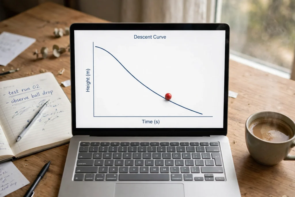
Gradient descent is the step-by-step method many machine learning models use to get better at a task. Instead of guessing the right settings once, the model checks its mistakes, adjusts its settings a little, and repeats the process until its predictions improve.
Key Takeaways
- Gradient descent reduces a model’s error by making small, repeated adjustments to its settings.
- The loss function measures how far predictions are from the correct answers.
- The learning rate controls how big each adjustment is: too large, and training can overshoot; too small, and it can crawl.
- Batch, stochastic, and mini-batch gradient descent differ mainly in how much data they use before each update.
- Good training also needs clean data, sensible settings, and honest checks on new examples.
What does gradient descent actually do?
Think of training as walking downhill in fog. You cannot see the whole valley, but you can feel the slope under your feet. If the ground slopes down to your left, you step left. If it slopes down to your right, you step right. Gradient descent works in a similar spirit: it looks at the slope of the error, then moves the model’s settings in the direction that should lower that error.
In machine learning, those settings are often called weights and biases. A weight decides how much attention the model pays to a particular input, while a bias shifts a prediction up or down. During training, gradient descent nudges these values again and again. Each nudge is small, but over many rounds the model can move from rough guesses to much more useful predictions.
That is why gradient descent sits at the heart of so much modern AI. It is not the model itself, and it is not the data. It is the learning routine that helps a model adjust itself, whether the task is predicting house prices, sorting photos, or recognising spoken words.
What is the loss function?
The loss function is the model’s scorecard. It compares what the model predicted with what actually happened, then turns the difference into a single number. A high loss means the predictions are still far off. A low loss means they are getting closer.
Different tasks use different loss functions. For a prediction task with numbers, such as estimating a price, the model might use mean squared error, which punishes large mistakes more heavily. For a sorting task, such as deciding whether a photo shows a cat or a dog, it might use a different loss that fits probabilities better. The details change, but the idea stays the same: training is about finding settings that bring loss down.
This is also where honest testing matters. A model can look excellent on the examples it trained on and still struggle with new ones. That is why model evaluation uses fresh data to check whether the improvement is real, rather than just memorised.

How does the learning rate change training?
The learning rate is the size of each step. Picture the foggy hillside again. With a sensible step size, you move steadily downhill and settle in the valley. With steps that are far too large, you might leap straight over the valley and land higher on the other side, then bounce back and forth without settling. With steps that are far too tiny, you will still head downhill, but the trip may take far longer than it needs to.
In practice, choosing a learning rate is a balancing act. A rate that is too high can make training unstable, with loss jumping around instead of falling. A rate that is too low can make training slow and may leave the model stuck before it reaches a good answer. Many training setups start with a moderate rate and reduce it as training goes on, so the model takes broader steps early and finer steps as it nears a good result.
It also helps to remember that the learning rate is not learned from the data in the same way as weights. It is a setting chosen before training, sometimes after a few experiments. If a model is not improving, the learning rate is one of the first settings worth checking — but it is rarely the only thing that matters. Data quality, model design, and the amount of training time all play a part.
What are batch, stochastic, and mini-batch gradient descent?
These three versions differ in how much data the model looks at before it updates its settings.
Batch gradient descent uses the whole training set for each update. That gives a steady, reliable sense of direction, because every example contributes to the decision. The downside is cost: for a large dataset, working through everything before a single update can be slow and memory-hungry.
Stochastic gradient descent, often shortened to SGD, updates after just one example at a time. That makes updates fast and frequent, and the extra randomness can sometimes help the model escape a shallow dip in the error landscape. The trade-off is noise: individual examples can pull the model in slightly different directions, so the path downhill looks bumpier.
Mini-batch gradient descent sits in between. It splits the data into small groups, or batches, and updates after each batch. This is the approach used most often in practice, because it balances speed, stability, and the efficient use of modern hardware. If you hear someone say they are training with SGD today, they often mean mini-batch gradient descent in practice.
None of these is automatically best for every job. The right choice depends on the size of the dataset, the hardware available, and how much noise the training process can tolerate.
Why can gradient descent get stuck?
A simple error landscape has one clear valley, called the global minimum. Many real problems are messier. They may have local minima: smaller dips that look like valleys but are not the lowest point overall. A model can settle into one and stop improving, even though a better answer exists elsewhere.
Saddle points cause a similar headache. At a saddle point, the slope is flat in one direction but not in others, so the model may slow down or stall even though it has not reached a good answer. In deep networks, very small gradients can also cause early layers to learn far more slowly than later ones, a problem known as vanishing gradients. The opposite problem, exploding gradients, can make updates so large that training becomes unstable.
These issues do not mean gradient descent is broken. They explain why training a complex model takes care, why researchers developed variations such as momentum and adaptive learning rates, and why a model that trains well on paper can still need tuning in practice. A good explanation of the core idea is available from IBM’s guide to gradient descent, and its companion guide covers stochastic gradient descent in more detail.
How does gradient descent fit into machine learning?
Gradient descent is a training tool, not a type of model on its own. It helps machine learning systems adjust their settings, and it is especially important in deep learning, where networks have many layers of weights to tune. In a neural network, a related method called backpropagation works out how much each weight contributed to the error, and gradient descent then uses that information to update the weights.
That combination is powerful, but it still depends on the basics. If the data is messy, biased, or unrepresentative, even a well-tuned training routine will learn the wrong lessons. If the model is far too complex for the amount of data available, it may memorise examples instead of learning patterns that generalise. Gradient descent can only optimise what it is given, so the quality of the data and the design of the model matter just as much as the training method.
This is also why gradient descent connects naturally to the broader story of AI. The complete guide to artificial intelligence explains how learning from data fits into the field as a whole, while gradient descent explains one of the main ways that learning actually happens, step by step.

A simple example to keep in mind
Imagine a model trying to predict the price of a used bicycle from its age and condition. At first, its weights are rough guesses, so its price estimates are often wrong. The loss function records those errors. Gradient descent then checks which direction would reduce the error, nudges the weights a little, and tries again.
After one round, the estimates may improve only slightly. After many rounds, the model may start to notice sensible patterns: older bikes tend to cost less, and bikes in better condition tend to cost more. It has not been handed those rules directly. It has found useful settings by repeatedly reducing its own errors.
That example is deliberately simple, and real models work with far more inputs and far messier data. Still, the loop is the same: predict, measure the error, adjust, repeat. When that loop is run carefully, with a sensible learning rate and honest checks on new data, gradient descent turns a rough starting model into one that is genuinely useful.
FAQs
Is gradient descent the same as machine learning?
No. Machine learning is the broader field of building systems that improve from data. Gradient descent is one optimisation method used to train many of those systems. Other training methods exist, but gradient descent is among the most widely used.
What happens if the learning rate is too high?
Training can become unstable. The model may overshoot the lowest point, bounce from side to side, and fail to settle. In extreme cases, the loss can grow instead of shrinking, which is a clear sign that the step size needs to be reduced.
What happens if the learning rate is too low?
Training becomes slow. The model still moves in the right direction, but each step is tiny, so it may need many more rounds to reach a good result. It can also get stuck more easily in a shallow dip before finding a better answer.
Do all models use gradient descent?
No, although many do. Some models, such as certain decision trees, are built with different methods. Gradient descent is most common for models with settings that can be adjusted smoothly, including linear models and neural networks.
Can gradient descent guarantee the best possible model?
Not always. For simple, convex problems, it can reliably find the best answer. For more complex problems, it may settle in a local minimum or a saddle point instead. That is why model design, data quality, and careful evaluation matter alongside the training method itself.
Conclusion
Gradient descent is best understood as a patient, practical routine: measure the error, find the downhill direction, take a sensible step, and repeat. The learning rate sets the step size, the loss function keeps score, and the choice of batch size shapes how noisy or steady the journey feels.
If you want a useful next step, try the idea on a tiny problem of your own. Pick one simple prediction task, watch how changing the step size changes the result, and check your model on examples it has never seen. That small experiment captures the heart of gradient descent better than any diagram: learning, in AI, is often just careful adjustment, repeated many times.